Search For Fun

A blog for collecting diverse useful information


  • Home

  • Tags

  • Categories

  • Archives

  • Search

R language to cluster image colors by using k-means clustering

Posted on 2018-09-27 | Edited on 2018-07-24 | In machine learning

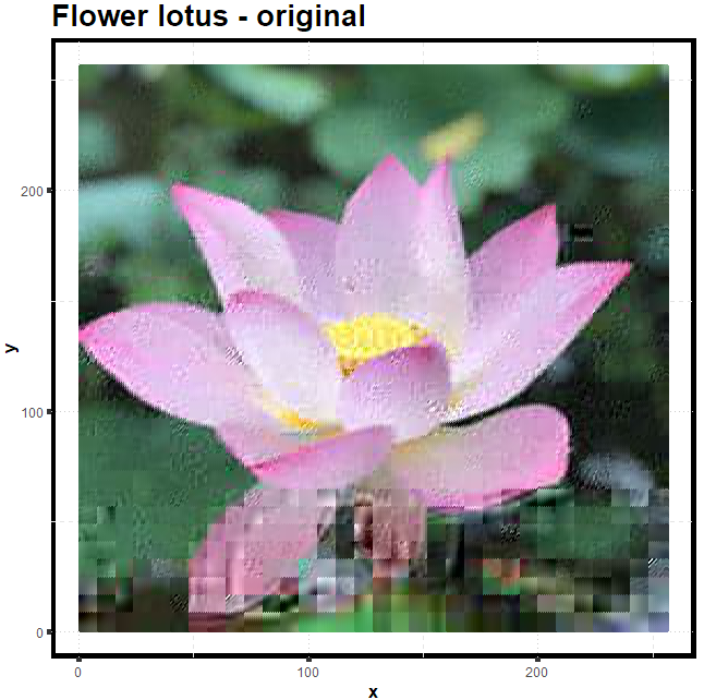
description: cluster colors in a flower image through k-means

downloading and reading image file

1
2
3
4
library("jpeg")
imageurl<-"https://thumbs-prod.si-cdn.com/WRp3AC1A1q3d4_lCe_fzfMmIu0o=/256x256/https://public-media.smithsonianmag.com/accounts/avatars/IMG_E1531.JPG"
dFile <- download.file(imageurl, "lotus.jpg") # download file to workspace
img <- readJPEG("lotus.jpg") # read local image

processing image data

1
2
3
4
5
6
7
8
9
10
imgDm <- dim(img)
imgDm # [1] 879 1200 3
imgRGB <- data.frame(
x = rep(1:imgDm[2], each = imgDm[1]),
y = rep(imgDm[1]:1, imgDm[2]),
R = as.vector(img[,,1]),
G = as.vector(img[,,2]),
B = as.vector(img[,,3])
)
imgRGB # X 1 y 879 R .. G .. B ..

set a theme for drawing the image

1
2
3
4
5
6
7
8
9
10
11
12
13
14
15
16
17
18
19
20
21
22
23
24
25
26
27
28
29
30
31
32
33
34
library(ggplot2)
plotTheme <- function(){
theme(
panel.background = element_rect(
size = 3,
colour = "black",
fill = "white"
),
axis.ticks = element_line(
size = 2
),
panel.grid.major = element_line(
colour = "gray80",
linetype = "dotted"
),
panel.grid.minor = element_line(
colour = "gray90",
linetype = "dashed"
),
axis.title.x = element_text(
size = rel(1.2),
face = "bold"
),
axis.title.y = element_text(
size = rel(1.2),
face = "bold"
),
plot.title = element_text(
size = 20,
face = "bold",
vjust = 1.5
)
)
}

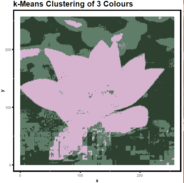
image clustering using K-means clustering

1
2
3
4
5
6
7
8
9
10
kClusters <- 3 
kMeans <- kmeans(imgRGB[,c("R","G","B")], centers = kCluster)
kColours <- rgb(kMeans$centers[kMeans$cluster,])

ggplot(data = imgRGB, aes(x = x, y = y)) +
geom_point(colour = kColours) +
labs(title = paste("k-Means Clustering of", kClusters, "Colours")) +
xlab("x") +
ylab("y") +
plotTheme()

outcome

R language to build ANN network for wine data

Posted on 2018-09-27 | Edited on 2018-07-23 | In machine learning

description: build ANN network from wine data in r language

read table data

1
2
3
4
wine <- read.table("https://archive.ics.uci.edu/ml/machine-learning-databases/wine/wine.data",
sep=",", # 分隔符为 , comma
col.names=c("Type","Alcohol","Malic","Ash","Alcalinity","Magnesium","Phenols","Flavanoids","Nonflavanoids","Proanthocyanins","Color","Hue","Dilution","Proline")
)

preview data

1
2
3
4
5
6
7
8
9
10
11
12
13
14
15
16
17
18
19
20
21
22
print(wine)
# Type Alcohol Malic Ash Alcalinity Magnesium Phenols Flavanoids
# 1 1 14.23 1.71 2.43 15.6 127 2.80 3.06
# 2 1 13.20 1.78 2.14 11.2 100 2.65 2.76
# 3 1 13.16 2.36 2.67 18.6 101 2.80 3.24
# 4 1 14.37 1.95 2.50 16.8 113 3.85 3.49
# 5 1 13.24 2.59 2.87 21.0 118 2.80 2.69
# ....

print(nrow(wine))
# [1] 178

print(ncol(wine))
# [1] 14

print(summary(wine))
# Type Alcohol Malic Ash
# Min. :1.000 Min. :11.03 Min. :0.740 Min. :1.360
# 1st Qu.:1.000 1st Qu.:12.36 1st Qu.:1.603 1st Qu.:2.210
# Median :2.000 Median :13.05 Median :1.865 Median :2.360
# Mean :1.938 Mean :13.00 Mean :2.336 Mean :2.367
# ...

attribute to categorical data

1
2
3
4
5
6
7
8
wine$Type=factor(wine$Type)
print(summary(wine))
# Type Alcohol Malic Ash Alcalinity
# 1:59 Min. :11.03 Min. :0.740 Min. :1.360 Min. :10.60
# 2:71 1st Qu.:12.36 1st Qu.:1.603 1st Qu.:2.210 1st Qu.:17.20
# 3:48 Median :13.05 Median :1.865 Median :2.360 Median :19.50
# Mean :13.00 Mean :2.336 Mean :2.367 Mean :19.49
# ...

data pre-processing and transformation

1
2
3
4
5
6
7
8
9
wine.scale <- cbind(wine[1], scale(wine[-1]))
print(summary(wine.scale))
apply(wine.scale[-1], 2, sd)
# Type Alcohol Malic Ash
# 1:59 Min. :-2.42739 Min. :-1.4290 Min. :-3.66881
# 2:71 1st Qu.:-0.78603 1st Qu.:-0.6569 1st Qu.:-0.57051
# 3:48 Median : 0.06083 Median :-0.4219 Median :-0.02375
# Mean : 0.00000 Mean : 0.0000 Mean : 0.00000
# ...

partitioning the data into training and test data

1
2
3
4
5
6
7
8
data.size <- nrow(wine.scale) 
set.seed(1111)
samp <- c(sample(1:data.size, data.size*0.7))
data.tr <- wine.scale[samp, ]
data.test <- wine.scale[-samp, ]

summary(data.tr)
summary(data.test)

data mining using a neural Network classification technique

1
2
3
4
5
6
7
8
9
10
11
12
13
library(nnet)
model.nnet <- nnet(Type ~ .,
data = data.tr,
size=2, # 2 level
decay=5e-04,
maxit=200) # stopped after 200 iterations
summary(model.nnet)
# initial value 164.152084
# iter 10 value 7.066118
# iter 20 value 1.286566
# iter 30 value 0.542334
# iter 40 value 0.444873
# ...

pattern (model) evaluation

1
2
3
4
5
6
7
8
9
10
11
12
13
14
15
16
predicted <- predict(model.nnet,
data.test,
type="class")
predicted

actual <- data.test$Type
model.confusion.matrix <- table(actual, predicted)
model.confusion.matrix

confusion.matrix.rate = prop.table(model.confusion.matrix) * 100
round(confusion.matrix.rate, digit=2)

diag.index <- cbind(1:3, 1:3)

error.overall = sum(confusion.matrix.rate) - sum(confusion.matrix.rate[diag.index])
paste("Error Rate =", round(error.overall, digit=2), "%")

Data mining Task using a nearest neighbour approach

1
2
3
4
5
6
7
8
9
10
11
12
13
14
15
16
17
18
19
20
21
22
P1=c(1,3) 
P2=c(2,4)
P3=c(6,6)

N1=c(2,1)
N2=c(5,3)
N3=c(6,4)

train=rbind(P1,P2,P3,N1,N2,N3) # build the classification matrix
plot(train)

class=factor(c(rep("lover",3),rep("hater",3))) # [1] lover lover lover hater hater hater
class

test=c(1,4) # testing data to be classified
test # 1 4

library(class)
summary(knn(train, test, class, k=3)) # hater 0 lover 1

test=c(6,4)
summary(knn(train, test, class, k=3)) # hater 1 lover 0

python numpy datetime64 today

Posted on 2018-09-27 | Edited on 2018-07-14 | In python

python numpy datetime64 today

1
2
3
4
5
6
7
8
9
10
11
12
13
14
15
16
>>> import numpy as np
>>> import datetime
>>> today = np.datetime64(datetime.datetime.now())
>>> today
numpy.datetime64('2018-07-12T19:12:39.167044')
>>> past = np.datetime64('2018-01-01')
>>> past
numpy.datetime64('2018-01-01')
>>> dif = today - past
>>> dif
numpy.timedelta64(16657959167044,'us')
>>> dif = np.timedelta64(dif, 'D')
>>> dif
numpy.timedelta64(192,'D')
>>> dif.astype(int)
192

more on searchfor.space

python timedelta to seconds

Posted on 2018-09-27 | Edited on 2018-07-14 | In python

python timedelta to seconds

1
2
3
4
5
6
7
8
9
10
11
12
13
14
15
16
17
import numpy as np 
import datetime

today = np.datetime64(datetime.datetime.today())
today
# numpy.datetime64('2018-07-12T19:28:08.889374')

past = np.datetime64('2018-07-11')
past
# numpy.datetime64('2018-07-11')

dif = today - past
dif
# numpy.timedelta64(156488889374,'us')

dif.astype(int)
# 1870066718

more on searchfor.space

python parse string into datetime

Posted on 2018-09-27 | Edited on 2018-07-20

description: python parse string into datetime

parse string into datetime

1
2
3
import datetime 
datetime.datetime.strptime('2018-01-01', "%Y-%m-%d")
# datetime.datetime(2018, 1, 1, 0, 0)

more on search4fan.github.io

python print format string example

Posted on 2018-09-27 | Edited on 2018-07-21 | In python

description: python print format string example

python Using % and .format() for formating print output

1
2
3
4
5
for i in range(1, 60):
interaction = '%s' % ('#' *i)
print('\r{}'.format(interaction), end='')
time.sleep(1)
# #############...

more on search4fan.github.io

python extract columns from dataframe

Posted on 2018-09-27 | Edited on 2018-07-22 | In python

description: pandas select columns by name

python select columns from dataframe by name

1
2
3
4
5
6
7
8
9
import pandas 
d = pandas.DataFrame([[1,2,3,4]], columns=['a','b','c','d'])
# d
# a b c d
# 0 1 2 3 4
d2 = d[['b','c']]
# d2
# b c
# 0 2 3

more on search4fan.github.io

python add one day to a date

Posted on 2018-09-27 | Edited on 2018-07-20 | In python

description: python add one day to a date

python datetime date add one day

1
2
3
4
5
6
import datetime
d = datetime.datetime.strptime('2018-02-01', '%Y-%m-%d')
# d
# datetime.datetime(2018, 2, 1, 0, 0)
d + datetime.timedelta(days=1)
# datetime.datetime(2018, 2, 2, 0, 0)

more on search4fan.github.io

python resign headers to a dataframe

Posted on 2018-09-27 | Edited on 2018-07-19

description: python pandas rename or change column names

python rename column headers

1
2
3
4
5
6
7
8
9
10
import pandas 
d1 = pandas.DataFrame([[1,2,3]])
# d1
# 0 1 2
# 0 1 2 3

d2 = pandas.DataFrame(d1.values, columns = ['a', 'b', 'c'])
# d2
# a b c
# 0 1 2 3

more on search4fan.github.io

python change dataframe column into set and loop the set

Posted on 2018-09-27 | Edited on 2018-07-20 | In python

description: change dataframe column into set and iterate

change dataframe column into a set

1
2
3
4
5
6
7
8
9
10
11
12
import pandas
a = pandas.DataFrame([[1,2],[2,3],[4,5]], columns=['a','b'])
# a
# a b
# 0 1 2
# 1 2 3
b = a['a'].unique()
# b
# array([1, 2, 4], dtype=int64)
b = set(b)
# b
# {1, 2, 4}

iterate dataframe column set

1
2
3
4
5
for item in b:
print(item)
# 1
# 2
# 4

combine into a single code

1
2
3
4
5
for item in a['a'].unique():
print(item)
# 1
# 2
# 4

more on search4fan.github.io

123…7

killfun

Personal blog for collecting useful information

64 posts
14 categories
38 tags
RSS
© 2018 killfun
Powered by Hexo v3.7.1
|
Theme — NexT.Muse v6.3.0